06. Gene Regulatory Network Inference#
This notebook will introduce the usage of gene regulatory network inference after fitting velocity model
[1]:
import pygot
import matplotlib.pyplot as plt
import seaborn as sns
import scanpy as sc
import numpy as np
plt.rc('axes.spines', top=False, right=False)
%matplotlib inline
loading simulation data and preprocess#
[2]:
adata = pygot.datasets.synthetic()
time_key = 'Day'
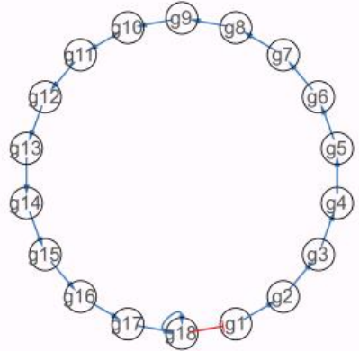
This data is generated from a gene regulatory network of 18 genes, which drives cells differentiate into three different cell type. The groundtruth stored in adata.uns[‘ref_network’] and the groundtruth velocity store in adata.layers[‘velocity_groundtruth’] The underlying GRN is
and show in the dataframe format
[3]:
ref_network = adata.uns['ref_network']
ref_network.head()
[3]:
| Gene2 | Gene1 | Type | |
|---|---|---|---|
| 0 | g3 | g2 | + |
| 1 | g5 | g4 | + |
| 2 | g18 | g17 | + |
| 3 | g18 | g18 | + |
| 4 | g1 | g18 | - |
[4]:
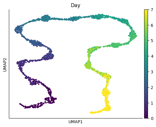
sc.pp.neighbors(adata)
sc.tl.umap(adata)
sc.pl.umap(adata, color=time_key)
OMP: Info #276: omp_set_nested routine deprecated, please use omp_set_max_active_levels instead.
Using VAE to perform non-linear dimension reduction#
we use VAE from pygot.pp.GS_VAE to train the VAE model. The inverse_transform function is already defined as vae.inverse_transform
[5]:
vae = pygot.preprocessing.GS_VAE()
vae.register_model(adata, latent_dim=2)
adata.obsm['X_latent'] = vae.fit_transform(adata, n_epoch=100)
To use VAE, run as following:
     1. gs_vae.register_model
     2. gs_vae.fit / gs_vae.fit_transform
To use GS-VAE, run as following:
     1. gs_vae.precompute_gs
     2. gs_vae.process_gs
     3. gs_vae.register_model
     4. gs_vae.fit / gs_vae.fit_transform
loss :68.2939: 100%|██████████| 100/100 [00:02<00:00, 33.52it/s]
In here, we train the velocity model in both orginal and vae space to infer the gene velocity. For vae model, we use the decoder of VAE and chain rule to obtain gene velocity via latent velocity.
[6]:
embedding_key = 'X_origin'
model_origin, history = pygot.tl.traj.fit_velocity_model(
            adata, time_key, embedding_key, v_centric_iter_n=500, x_centric_iter_n=1000)
loading saved shortest path profile
[Errno 2] No such file or directory: '/_0.0to1.0.pkl'
Error in loading shortest path file
calcu shortest path between 0.0 to 1.0
100%|██████████| 375/375 [00:00<00:00, 2142.55it/s]
calcu shortest path between 1.0 to 2.0
100%|██████████| 375/375 [00:00<00:00, 4310.63it/s]
calcu shortest path between 2.0 to 3.0
100%|██████████| 375/375 [00:00<00:00, 4260.35it/s]
calcu shortest path between 3.0 to 4.0
100%|██████████| 375/375 [00:00<00:00, 4096.47it/s]
calcu shortest path between 4.0 to 5.0
100%|██████████| 375/375 [00:00<00:00, 4222.01it/s]
calcu shortest path between 5.0 to 6.0
100%|██████████| 375/375 [00:00<00:00, 4256.19it/s]
calcu shortest path between 6.0 to 7.0
100%|██████████| 375/375 [00:00<00:00, 4390.79it/s]
loss :0.5285 best :0.5285: 100%|██████████| 500/500 [01:28<00:00,  5.64it/s]
loss :9.0808  best :9.0808: 100%|██████████| 1000/1000 [00:20<00:00, 47.96it/s]
[7]:
embedding_key = 'X_latent'
model_latent, history = pygot.tl.traj.fit_velocity_model(
            adata, time_key, embedding_key, v_centric_iter_n=500, x_centric_iter_n=1000)
loading saved shortest path profile
[Errno 2] No such file or directory: '/_0.0to1.0.pkl'
Error in loading shortest path file
calcu shortest path between 0.0 to 1.0
100%|██████████| 375/375 [00:00<00:00, 3645.69it/s]
calcu shortest path between 1.0 to 2.0
100%|██████████| 375/375 [00:00<00:00, 3592.54it/s]
calcu shortest path between 2.0 to 3.0
100%|██████████| 375/375 [00:00<00:00, 4230.13it/s]
calcu shortest path between 3.0 to 4.0
100%|██████████| 375/375 [00:00<00:00, 4304.70it/s]
calcu shortest path between 4.0 to 5.0
100%|██████████| 375/375 [00:00<00:00, 4148.00it/s]
calcu shortest path between 5.0 to 6.0
100%|██████████| 375/375 [00:00<00:00, 4152.23it/s]
calcu shortest path between 6.0 to 7.0
100%|██████████| 375/375 [00:00<00:00, 4220.58it/s]
loss :0.1151 best :0.1151: 100%|██████████| 500/500 [00:38<00:00, 13.03it/s]
loss :0.7151  best :0.7082: 100%|██████████| 1000/1000 [00:21<00:00, 46.66it/s]
Comparsion velocity accuracy between origin and VAE space#
After training, we can transform the latent velocity into 2-d umap velocity to velocity. Both the umap velocity obtained from origin and vae are very close to groundtruth velocity.
[8]:
import scvelo as scv
fig, axs = plt.subplots(1,3, figsize=(16, 5))
adata.layers['velocity'] = adata.layers['velocity_groundtruth']

adata.layers['Ms'] = adata.X
scv.tl.velocity_graph(adata)
true_latent_v = adata.layers['velocity'] @ adata.varm['PCs']
scv.pl.velocity_embedding_grid(adata, basis='umap',
                                        ax=axs[0], arrow_size=2, arrow_length=2, color=time_key, show=False, title='Ground Truth')

#origin
embedding_key = 'X_origin'
origin2gene_velocity = pygot.tl.traj.velocity(adata, model_origin.func, time_key=time_key, embedding_key=embedding_key, A=np.eye(adata.shape[1]))
adata.layers['velocity'] = origin2gene_velocity
pygot.tl.traj.velocity_graph(adata, embedding_key=embedding_key, velocity_key='velocity_origin')
del adata.obsm['velocity_umap']
scv.pl.velocity_embedding_grid(adata, basis='umap', ax=axs[1], arrow_size=2, arrow_length=2,color=time_key, show=False, title='Predicition (Origin)')


#vae
embedding_key = 'X_latent'
vae2gene_velocity = pygot.tl.traj.velocity(adata, model_latent.func, embedding_key=embedding_key, time_key=time_key, dr_mode='nonlinear', inverse_transform=vae.inverse_transform)
adata.layers['velocity'] = vae2gene_velocity
pygot.tl.traj.velocity_graph(adata, embedding_key=embedding_key, velocity_key='velocity_latent')
del adata.obsm['velocity_umap']
scv.pl.velocity_embedding_grid(adata, basis='umap', ax=axs[2], arrow_size=2, arrow_length=2, color=time_key, show=False, title='Predicition (VAE)')
computing velocity graph (using 1/10 cores)
WARNING: Unable to create progress bar. Consider installing `tqdm` as `pip install tqdm` and `ipywidgets` as `pip install ipywidgets`,
or disable the progress bar using `show_progress_bar=False`.
    finished (0:00:00) --> added
    'velocity_graph', sparse matrix with cosine correlations (adata.uns)
computing velocity embedding
    finished (0:00:00) --> added
    'velocity_umap', embedded velocity vectors (adata.obsm)
Use adata.obsp['connectivities'] as neighbors, please confirm it is computed in embedding space
computing velocity embedding
    finished (0:00:00) --> added
    'velocity_umap', embedded velocity vectors (adata.obsm)
Use adata.obsp['connectivities'] as neighbors, please confirm it is computed in embedding space
computing velocity embedding
    finished (0:00:00) --> added
    'velocity_umap', embedded velocity vectors (adata.obsm)
[8]:
<Axes: title={'center': 'Predicition (VAE)'}>
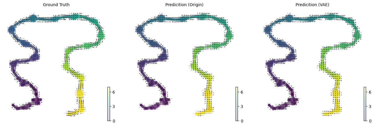
Next, we compare the gene velocity directly infered from original space / the recovered gene velocity from vae space with groundtruth gene velocity
[9]:
true_velo = adata.layers['velocity_groundtruth']
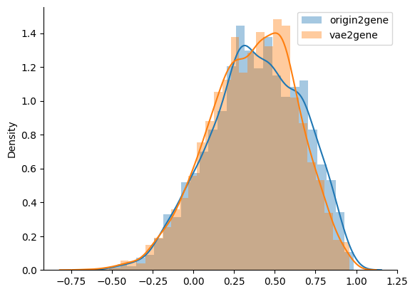
Significantly, they have comparable accuracy
[10]:
cos_similarity_with_pca = np.sum(origin2gene_velocity * true_velo, axis=1) / (np.linalg.norm(origin2gene_velocity, axis=1)*np.linalg.norm(true_velo, axis=1))
cos_similarity_with_vae = np.sum(vae2gene_velocity * true_velo, axis=1) / (np.linalg.norm(vae2gene_velocity, axis=1)*np.linalg.norm(true_velo, axis=1))
sns.distplot(cos_similarity_with_pca, label='origin2gene')
sns.distplot(cos_similarity_with_vae, label='vae2gene')
plt.legend()
[10]:
<matplotlib.legend.Legend at 0x32ca68910>
Gene regulatory network inference#
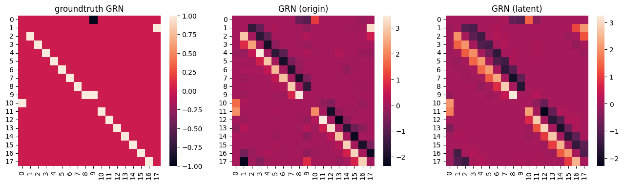
Finally, we can use the gene velocity to construct a regression model to infer the gene regulatory network (GRN), and evalute the performance by compute area under curve of precision and recall (AUCPR) value between groundtruth GRN and infered GRN.
[11]:
grn = pygot.tl.analysis.GRN()
adata.layers['velocity'] = pygot.tl.traj.latent_velocity(adata, model_origin.func, embedding_key='X_origin', time_key=time_key)
grn_data_origin = grn.fit(adata, TF_constrain=False, non_negative=False)
print('PR:', pygot.evalute.compute_pr(adata.uns['ref_network'], grn_data_origin.ranked_edges))
TF number: 18, Index(['g1', 'g10', 'g11', 'g12', 'g13', 'g14', 'g15', 'g16', 'g17', 'g18',
       'g2', 'g3', 'g4', 'g5', 'g6', 'g7', 'g8', 'g9'],
      dtype='object')
scale velocity with factor : 3.0845143883801915
l1_penalty: 0.005 min_beta: 1.0
Epoch [6943/10000], Train Loss: 2.6323, Val Loss: 1.3067: 69%|██████▉ | 6943/10000 [00:08<00:03, 801.70it/s]
Early stopping at epoch 6944. Best validation loss: 1.30654
PR: 0.934571702244116
[12]:
grn = pygot.tl.analysis.GRN()
adata.layers['velocity'] = vae2gene_velocity
grn_data_latent = grn.fit(adata, TF_constrain=False, non_negative=False)
print('PR:', pygot.evalute.compute_pr(adata.uns['ref_network'], grn_data_latent.ranked_edges))
TF number: 18, Index(['g1', 'g10', 'g11', 'g12', 'g13', 'g14', 'g15', 'g16', 'g17', 'g18',
       'g2', 'g3', 'g4', 'g5', 'g6', 'g7', 'g8', 'g9'],
      dtype='object')
scale velocity with factor : 3.1818997927513477
l1_penalty: 0.005 min_beta: 1.0
Epoch [6424/10000], Train Loss: 2.0883, Val Loss: 1.0623: 64%|██████▍ | 6424/10000 [00:08<00:04, 772.85it/s]
Early stopping at epoch 6425. Best validation loss: 1.06216
PR: 0.9223086330116774
The infered GRNs are accurate and with high and close AUCPR value
[13]:
ref_matrix = np.zeros(shape=(len(adata.var), len(adata.var)))
ref_matrix[adata.var.loc[adata.uns['ref_network'].loc[adata.uns['ref_network']['Type'] == '+'].Gene2.tolist()]['idx'].tolist(),
           adata.var.loc[adata.uns['ref_network'].loc[adata.uns['ref_network']['Type'] == '+'].Gene1.tolist()]['idx'].tolist()] = 1

ref_matrix[adata.var.loc[adata.uns['ref_network'].loc[adata.uns['ref_network']['Type'] == '-'].Gene2.tolist()]['idx'].tolist(),
           adata.var.loc[adata.uns['ref_network'].loc[adata.uns['ref_network']['Type'] == '-'].Gene1.tolist()]['idx'].tolist()] = -1
Visualization of GRN
[14]:
fig, axes = plt.subplots(1,3, figsize=(16,4))
sns.heatmap(ref_matrix, ax=axes[0])
axes[0].set_title('groundtruth GRN')
sns.heatmap(grn_data_origin.G, ax=axes[1])
axes[1].set_title('GRN (origin)')
sns.heatmap(grn_data_latent.G, ax=axes[2])
axes[2].set_title('GRN (latent)')
[14]:
Text(0.5, 1.0, 'GRN (latent)')